A
Breath of Fresh Air
New
Mexico Supercomputing Challenge
Final
Report
April
4, 2013
Team
63
Los
Alamos Middle School
Los
Alamos, NM
Team
Members: Alex Bullock, Ryan Swart
Teacher: Mrs.Stephens
Project
Mentor: Pieter Swart
Executive Summary
The issue of global warming
has become a major concern as well as a political hot potato and this project
aims to provide education and insight by using high-quality data and scientific
visualization.
Our goal was to find and
understand a single, reliable source of data for the world-wide change in the
most important man-made greenhouse gas CO2. We then wrote an
interactive program to analyze and visualize this change so as to provide new
insights.
We found the
highest-quality data set for CO2
density to be that measured by the NASA AIRS instrument. We downloaded and
analyzed monthly measurements, and successfully visualized it using the
Processing language.
We found that
interactive exploration was very important to both debug the program and
understand the data.
Even over a
period as short as one decade, the user of this program can clearly see
significant global increases in CO2
densities in both the Northern and Southern hemispheres.
Seasonal variations
in CO2 concentrations are
also clearly visible, and we are researching whether one can see effects of
continent-wide forest fires in CO2
measurements as viewed from space.
Background
About 97
percent of climate scientists agree that human-made global warming is happening,
and that it is largely due to excessive levels of greenhouse gases being
released by a fast-growing population. It is unclear whether this will be
merely a minor and easily fixed problem, or whether it will turn into the most
serious problem of this century.
Without an atmosphere, the temperature of our
earth would be approximately -18°C ( 0°F). Our atmosphere increases the average temperature to a much warmer
14.4°C (57.9°F). After millions of years, it has stabilized to a composition of
78.09% Nitrogen, 20.95% Oxygen, around 1.25% water vapor, 0.93% Argon, 0.03% CO2, followed by traces of other gases. If this composition is disturbed, our
ecosystem and climate would be dramatically different (imagine a hot Venus
versus a chilly Mars). The (so-called) greenhouse gases act to block the escape
of heat from Earth in the form of long-wave infra-red radiation. Both Oxygen
and Nitrogen are practically invisible to infra-red radiation, but CO2 and water vapor are very good at blocking
infra-red radiation, and this fact together with their abundance make
them the two most important greenhouse gases. The
amount of water vapor is not much changed by humans, but ever since the industrial
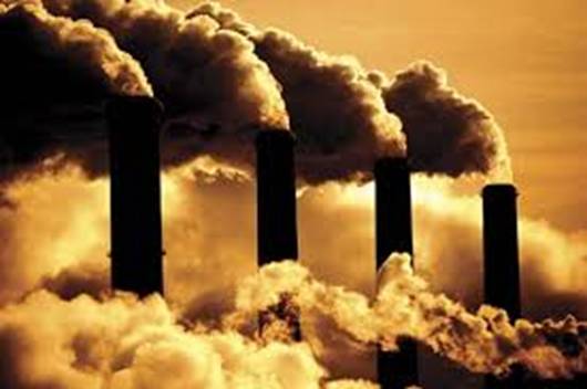
age we have been pumping enormous amounts of CO2 into our atmosphere. In this project we study CO2
as the most important greenhouse gas that is a by-product of human activities
such as: burning fossil fuels and biomass, and manufacturing concrete.
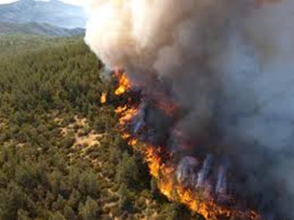
Forest fires also produce large amounts of CO2 each year, especially in developing countries where they start each spring and can spread through continents
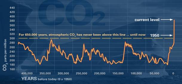
The figure below shows the rise and fall of CO2 levels over the past 650,000 years, as measured from
ancient air pockets in Antarctic ice cores [ Lűthi
et al.]. Since the 1950s CO2 has been growing in lockstep with the human population and GDP, has
broken the 300 parts per million (ppm) level record of the past 650,000 years,
and at this rate of growth could double by 2050. The question is how drastic
the consequences will be; will it be merely a storm in a teacup or will it
start a global economic and agricultural disaster?
Our initial goal for this
project was to collect and understand reliable data on the change in CO2 across the world, to
visualize it, and then to model and simulate pollutant (including smog and CO2) buildup and spread over
large cities and regions. However, a Google search on “CO2” and
“data” showed more
than 80 million hits. It was clearly impossible to sift through all of this to
determine who is right and who is wrong. This is also a major problem for the
general public and is responsible for many false
truths that confuses the discussion of global warming,
such as false assumptions like: "In one volcano eruption more CO2 is released than the
entire human race has emitted in their entire existence.” We therefore changed our
question due to this vast amount of confusing data and opinions, and our lack
of time to go through all of it. After looking at all our obstacles, we decided
we were going to take a different path and focus only on the first part of our
original goal.
Problem Statement
Our goal is to find a
single, reliable source of data for the world-wide change in CO2,
and write an interactive program to analyze and visualize this change so as to
provide new insights. By building a
website that runs this visualization, anyone anywhere in the world can rapidly
understand the data without being confused by the wide variety of largely political
opinions.
Data Sources
After a search for various
sources of CO2
data, we finally decided to use the NASA AIRS CO2
data in our project.
The Atmospheric Infrared
Sounder (AIRS) is an instrument on the NASA Aqua satellite whose mission is to
look at the density of important gases in the mid-troposphere (approximately
10km above the surface of earth).
AIRS was launched into Earth-orbit on May 4, 2002 and is one of six instruments on-board the Aqua satellite, part of the NASA Earth Observing System.
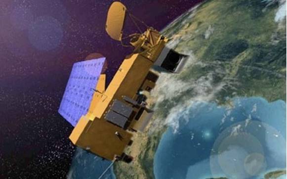
The Aquas satellite with the AIRS instrument on board.
AIRS uses cutting-edge
infrared technology to daily create large data sets that characterize
greenhouse gases. It can measure CO2 and
water vapor plus other trace greenhouse gases such as ozone, carbon monoxide,
and methane. With 2378 spectral channels it can collect more data about
greenhouse gases than any other satellite, and it can do it globally. Our
research shows this to be the best current source for CO2
data. On the AIRS website it states that “studies
have shown AIRS has improved global weather prediction more than any other
single satellite instrument in the past 10 years.”
The AIRS website provides
daily, weekly, and monthly-averaged measurements. We use the monthly-averaged
data because it is more accurate with fewer missing readings of data. The data
can be downloaded in HDF5 format from (http://mirador.gsfc.nasa.gov/cgibin/mirador/collectionlist.pl?keyword=airxc2m).
The HDF5 Data Format
HDF5 stands for Hierarchical Data Format
(version 5) and is mainly used for storing and reading large data sets. HDF5 is
an international standard and is designed to store high volume and complex data
sets together with its documentation as a compressed file system. It is used by
all NASA satellites, as well as many other satellites and observatories. The HDFView program (see http://www.hdfgroup.org for
a free download of this software) includes elementary tools and applications
for managing, manipulating, viewing, and analyzing data in the HDF5 data
format. We used this program to analyze our data in the following way:
We downloaded the monthly-averaged CO2
measurements from the NASA AIRS website in HDF5 format. We then used the
HDF5View software to convert the data into ASCII. This was imported into Excel
and reformatted as CSV (Comma Separated Values format) files, and the latter
was read as input by our Processing program. (It would have been much easier if
we had a Processing language library that could read HDF5 data files, but we
could not find one.)
NASA Datasets
The downloadable data from
the AIRS website (http://airs.jpl.nasa.gov/data/get_airs_co2_data/) is available in several different formats. We used the monthly level 3
data because of the higher quality and fewer missing data points. This data is
binned in 1x1 latitude-longitude degree bins, as shown below with HDFview.
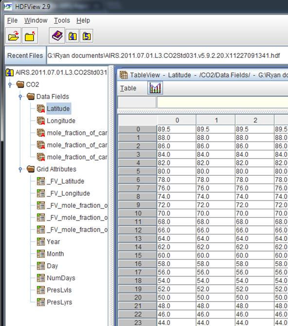
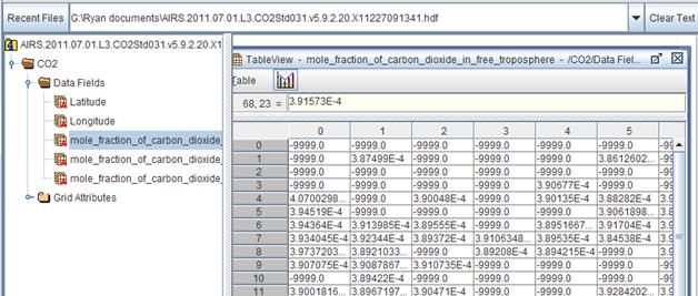
The CO2 concentration data
is measured in parts per million and organized in, the same 1x1 degree bins, as
shown in the screenshot below. Note the file system layout and the missing data
indicators.
These monthly data sets are
available for every month starting October 2002. We downloaded and converted
each monthly average data set, and stored the results in CSV files in folders
that are sorted by year and by month. In this wway
large data sets can be saved on disk and not in memory, thereby this program
should be able to cope with much larger data sets.
Software
We used the Processing language, designed by
Casey Reas & Ben Fry, in 2001, at MIT. Processing
is a visual, interactive language that borrows from Java. The code is open
source and available for many architectures at http://processing.org.
Processing is becoming very popular with artists and graphic designers for
visualizations. There are many libraries and books available, and we learned
most of our skills from openprocessing.org. It is outstanding for animation,
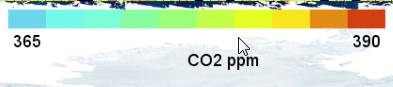
which is why we are using it. We also used a powerful library called ControlP5. ControlP5
is a Graphical User Interface (GUI) Processing library (http://www.sojamo.de/libraries/controlP5/)
that provides the ability to interactively change variables while running a
Processing program. For example, this can be shown as sliding bars. This is
very useful for interactively changing the year and month of the data set and
choosing the best visualization format in our program.
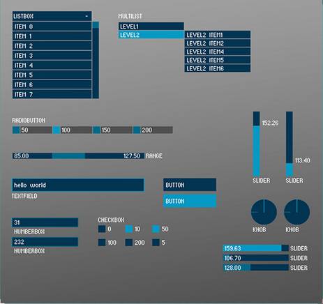
Example
of ControlP5 GUI Controllers
Adapting to Missing or Poor Data
The AIRS satellite does not
always record highly accurate data. The first reason is due to the fact that it
uses infrared channels to determine CO2
levels, and that these measurements are blocked by excessive cloud cover.
Secondly, as shown below, the satellite orbits the Earth from North to South
while scanning the troposphere. The cause of bad data at the poles is due to
the fact that often there is not enough sunlight at the poles for high accuracy
measurements. AIRS indicates inaccurate data measurements with the value of
-9999. Henceforth, in our visualization, we indicate incorrect data by black
squares (see figure below). In most of the data sets that we analyzed, the
incorrect or missing data are located around the North and South poles and the
Himalayas.
We use the function isGoodData() (see below) to change many algorithms, for example, the code to
calculate the maximum and minimum CO2
levels in a dataset that must exclude the -9999 values and uses this function
to do so.

boolean isGoodData(float x) {
// returns true if not very close
to -9999.0
if ( x > -9998.999 || x < -9999.0001 ) return true;
else return false;
}
In this example black rectangles
indicate where AIRS data is missing or of low precision, in this case over the
Arctic, the Norwegian Sea and the Himalayas. An example of how we cope with bad data is shown in the code
snippet above.
Our Program
Our program evolved through at
least 11 major versions. Like a typical Processing program it has a setup and a
draw section, with the draw section repeating at a high frame rate to make
interactive visualization possible. See outline below and attached code for
more details. Unfortunately there are many processed data files that are too
large to be included with this report.

setup:
setup GUI using
ControlP5
define heatmap colors
select and load
year & month csv files
read latitude,
longitude, co2 data & convert to screen location
using
geoToPixel() function, store in matrix
draw:
set background map
read co2min &
co2max from sliders
for each 1x1 grid rect:
if bad data, then
draw black rect at screen location
else: calc color using heat map, draw rect
at screen location
repeat draw section
while interactively changing some
visualization
parameters
Pseudocode outline of our program
An advantage of
this approach is that one can interactively tune the visualization as well as
explore the data. We found that the choice of effective colors is very
important to making it possible to see small changes.
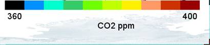
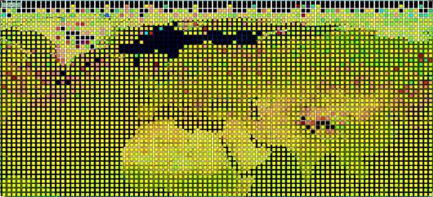
The above figure shows an example
heat map indicating CO2
concentration. In the end we used a color matcher to get as close as possible
to the colors used by the AIRS team. The final heat map is shown below.
Results
We first show below
how our visualization compared with the high-resolution NASA visualization of a
July 2008 CO2 intensity
measurement (shown below). We reproduced a rough copy of the NASA heat map. We
expect the data used by NASA to be of higher quality than what was available to
us. Also, we are not doing any smoothing of the data below. This comparison
shows that we are on the right path.
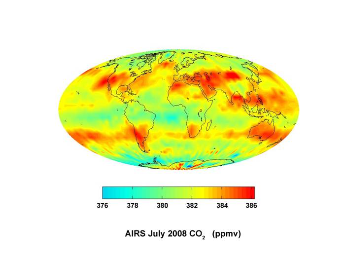
High resolution NASA visualization of a July
2008 CO2 intensity
measurement using AIRS.
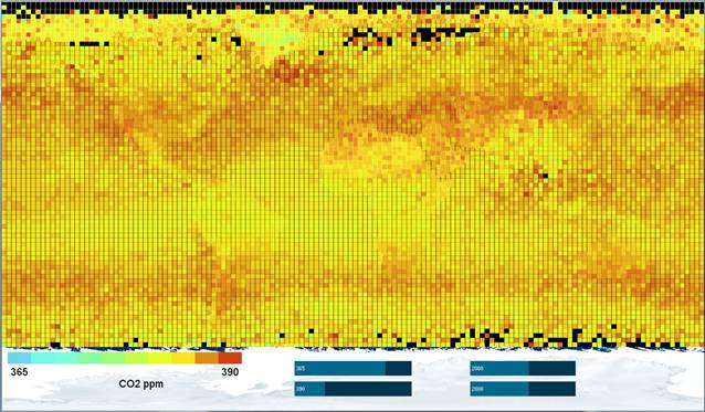
The above Figure
shows our visualization of the L3 monthly averaged CO2 intensities for July 2008, using a Mercator projection.
Note the black rectangles showing missing data. Continents are vaguely outlined
but some of these outlines are due to the underlying map showing through. When
making the rectangles slightly smaller but with everything else unchanged, as
shown below, the colors of the map show through and make some data points
darker/lighter than in reality. It turns out to be very hard to create a good
black outline map that will not bias the interpretation of data while still
showing the continents. Overall though, we see a good match with the NASA
image.
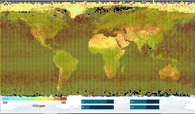
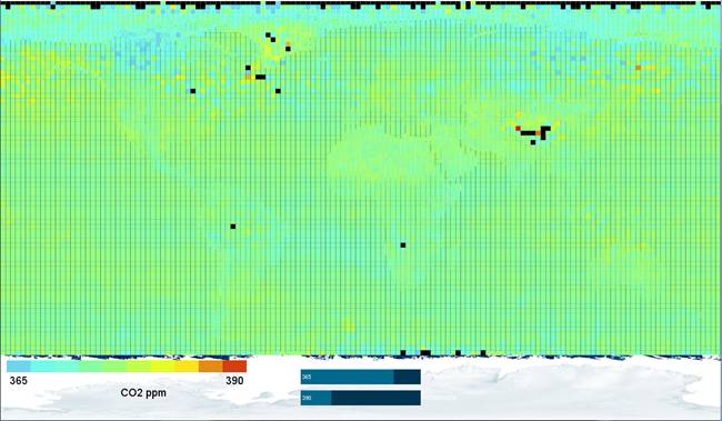
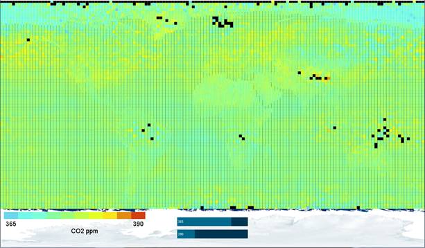
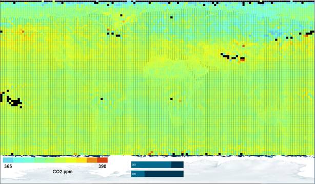
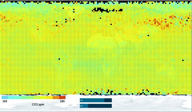
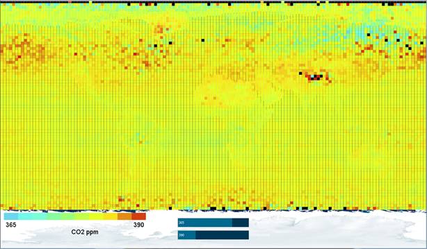
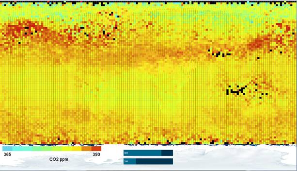
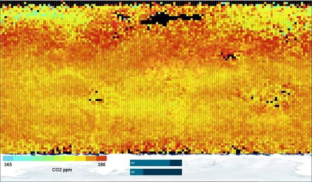
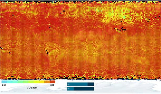
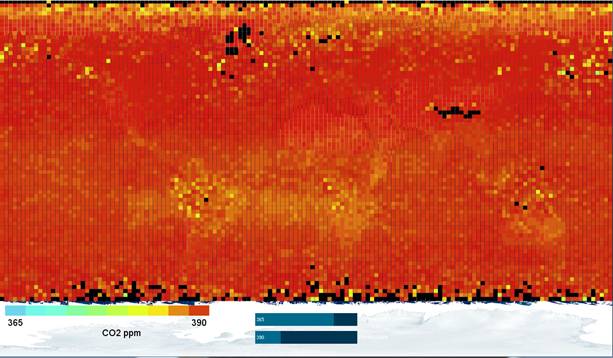
The next figures
show monthly-averaged CO2
concentration as measured by the NASA AIRS instrument during February for the
years 2003 to 2012. The heat map is chosen to be the same in
each visualization so that data can be compared between the years. An
increase in CO2 levels
can be seen in both hemispheres.
CO2 concentration in ppm
for Feb 2003 (monthly averaged) as measured by NASA AIRS instrument (black
indicates missing data)
CO2 concentration in ppm
for Feb 2004 (monthly averaged) as measured by NASA AIRS instrument (black
indicates missing data)
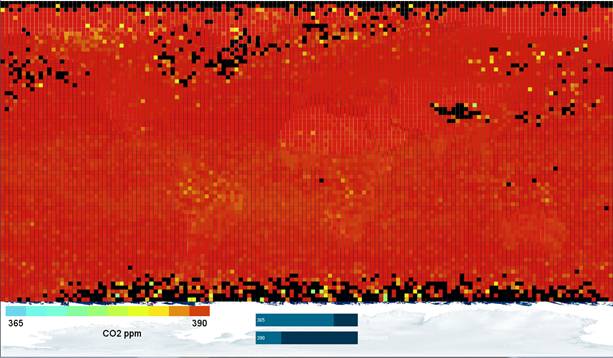
CO2 concentration in ppm
for Feb 2005 (monthly averaged) as measured by NASA AIRS instrument (black
indicates missing data)
CO2 concentration in ppm
for Feb 2006 (monthly averaged) as measured by NASA AIRS instrument (black
indicates missing data)
CO2 concentration in ppm
for Feb 2007 (monthly averaged) as measured by NASA AIRS instrument (black
indicates missing data)
CO2 concentration in ppm
for Feb 2008 (monthly averaged) as measured by NASA AIRS instrument (black
indicates missing data)
CO2 concentration in ppm
for Feb 2009 (monthly averaged) as measured by NASA AIRS instrument (black
indicates missing data)
CO2 concentration in ppm
for Feb 2010 (monthly averaged) as measured by NASA AIRS instrument (black
indicates missing data)
CO2 concentration in ppm
for Feb 2011 (monthly averaged) as measured by NASA AIRS instrument (black
indicates missing data)
CO2 concentration in ppm
for Feb 2012 (monthly averaged) as measured by NASA AIRS instrument (black
indicates missing data)
Conclusions
-
We found the highest-quality data set for CO2 density to be that measured by the NASA AIRS instrument.
We downloaded and analyzed monthly measurements, and successfully visualized it using the Processing language.
Interactive exploration was very important to debug the program and understand the data.
Even over a period as short as one decade, the user of this program will be able see the global changes in CO2 densities in both the Northern and Southern hemispheres.
Seasonal variations in CO2 concentrations are clearly visible, and we are researching whether one can see effects of continent-wide forest fires in CO2 measurements as viewed from space.
Most Original Achievement
We consider our
most original achievement the surprisingly large amount of change that can be
observed over such a short period of time. We also wrote software that
visualizes the difference between two data sets, and allows the user of this
program to compare the differences between any two months or years. This
ability is very useful because you can see the CO2 difference change in a
single area or a very large region. At this time we are still studying these
results and plan to publish it on our website.
References
·
http://www.ARL.NOAA.gov/smoke.php (December 4, 2012)
·
http://airs.jpl.nasa.gov/ (April 2, 2013)
·
Richter, Burton. Beyond Smoke and
Mirrors: Climate Change and Energy in the 21st Century. Cambridge, UK:
Cambridge UP, 2010. Print www.ARL.NOAA.gov/smoke.php
·
Casey Reas
and Ben Fry, Processing, MIT Press, 2007.
·
processing.org (December 4, 2012)
·
http://www.openprocessing.org/
(December 4, 2012)
·
High-resolution carbon dioxide
concentration record 650,000–800,000 years before present. D. Lűthi et al., Nature 453, 379-382
(15 May 2008)
Acknowledgements
We would like to thank:
Pieter
Swart for:
Helping us with our reports and when we got stuck.
Giving us inspiration.
All
the people that organized the supercomputing challenge.
The NM Supercomputing .judges, for their advice and
feedback during the Project Evaluation period and which significantly improved
our project.